Row-level geo-partitioning
Row-level geo-partitioning allows fine-grained control over pinning data in a user table (at a per-row level) to geographic locations, thereby allowing the data residency to be managed at the table-row level. Use-cases requiring low latency multi-region deployments, transactional consistency semantics, and transparent schema change propagation across the regions would benefit from this feature.
Geo-partitioning allows you to move data closer to users to:
- achieve lower latency and higher performance
- meet data residency requirements to comply with regulations such as GDPR
Geo-partitioning of data enables fine-grained, row-level control over the placement of table data across different geographical locations. This is accomplished in two steps:
- Partition a table into user-defined table partitions.
- Pin these partitions to the desired geographic locations by configuring metadata for each partition.
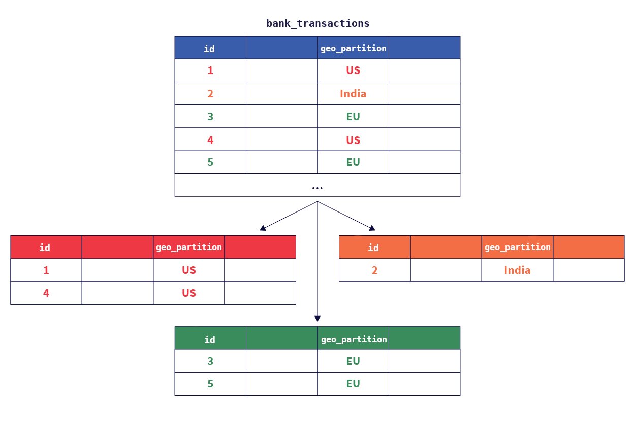
To create user-defined table partitions, designate a column of the table as the partition column that will be used to geo-partition the data. The value of this column for a given row is used to determine the table partition that the row belongs to.
The second step involves creating partitions in the respective geographic locations using tablespaces. Note that the data in each partition can be configured to get replicated across multiple zones in a cloud provider region, or across multiple nearby regions or data centers.
An entirely new geographic partition can be introduced dynamically by adding a new table partition and configuring it to keep the data resident in the desired geographic location. Data in one or more of the existing geographic locations can be purged efficiently by dropping the necessary partitions. Users of traditional RDBMS would recognize this scheme as being close to user-defined list-based table partitions, with the ability to control the geographic location of each partition.
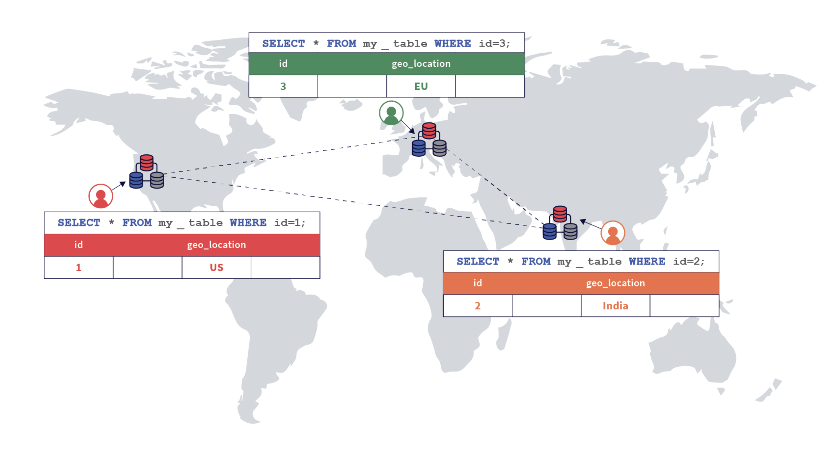
In this deployment, users can access their data with low latencies because the data resides on servers that are geographically close by, and the queries do not need to access data in far away geographic locations.
This tutorial explains this feature in the context of an example scenario described in the next section.
Example scenario
Suppose a large but imaginary bank, Yuga Bank, wants to offer an online banking service to users in many countries by processing their deposits, withdrawals, and transfers.
The following attributes would be required to build such a service:
- Transactional semantics with high availability: Consistency of data is paramount in a banking application, hence the database should be ACID compliant. Additionally, users expect the service to always be available, making high availability and resilience to failures a critical requirement.
- High performance: The online transactions need to be processed with a low latency in order to ensure a good end-user experience. This requires that the data for a particular user is located in a nearby geographic region. Putting all the data in a single location in an RDBMS would mean the requests for users residing far away from that location would have very high latencies, leading to a poor user experience.
- Data residency requirements for compliance: Many countries have regulations around which geographic regions the personal data of their residents can be stored in, and bank transactions being personal data are subject to these requirements. For example, GDPR has a data residency stipulation which effectively requires that the personal data of individuals in the EU be stored in the EU. Similarly, India has a requirement issued by the Reserve Bank of India (or RBI for short) making it mandatory for all banks, intermediaries, and other third parties to store all information pertaining to payments data in India – though in case of international transactions, the data on the foreign leg of the transaction can be stored in foreign locations.
Note
While this scenario has regulatory compliance requirements where data needs to be resident in certain geographies, the exact same technique applies for the goal of moving data closer to users to achieve low latency and high performance. Hence, high performance is listed above as a requirement.Step 1. Create tablespaces
First, create tablespaces for each geographic region you wish to partition data into:
-
Create tablespaces for each region.
CREATE TABLESPACE eu_central_1_tablespace WITH (
  replica_placement='{"num_replicas": 3, "placement_blocks":
  [{"cloud":"aws","region":"eu-central-1","zone":"eu-central-1a","min_num_replicas":1},
  {"cloud":"aws","region":"eu-central-1","zone":"eu-central-1b","min_num_replicas":1},
  {"cloud":"aws","region":"eu-central-1","zone":"eu-central-1c","min_num_replicas":1}]}'
);

CREATE TABLESPACE us_west_2_tablespace WITH (
  replica_placement='{"num_replicas": 3, "placement_blocks":
  [{"cloud":"aws","region":"us-west-2","zone":"us-west-2a","min_num_replicas":1},
  {"cloud":"aws","region":"us-west-2","zone":"us-west-2b","min_num_replicas":1},
  {"cloud":"aws","region":"us-west-2","zone":"us-west-2c","min_num_replicas":1}]}'
);

CREATE TABLESPACE ap_south_1_tablespace WITH (
  replica_placement='{"num_replicas": 3, "placement_blocks":
  [{"cloud":"aws","region":"ap-south-1","zone":"ap-south-1a","min_num_replicas":1},
  {"cloud":"aws","region":"ap-south-1","zone":"ap-south-1b","min_num_replicas":1},
  {"cloud":"aws","region":"ap-south-1","zone":"ap-south-1c","min_num_replicas":1}]}'
);
To view your tablespaces, you can enter the following command:
SELECT * FROM pg_tablespace;
Step 2. Create table with partitions
Next, create the parent table that contains a geo_partition column which is used to create list-based partitions for each geographic region you want to partition data into as shown in the following diagram:

-
Create the parent table.
CREATE TABLE bank_transactions (
    user_id   INTEGER NOT NULL,
    account_id INTEGER NOT NULL,
    geo_partition VARCHAR,
    account_type VARCHAR NOT NULL,
    amount NUMERIC NOT NULL,
    txn_type VARCHAR NOT NULL,
    created_at TIMESTAMP DEFAULT NOW()
) PARTITION BY LIST (geo_partition);
Note
You can set geo_partition to be DEFAULT yb_server_region() to partition based on regions. This way, insertions to the local partitioned table don't have to specify the geo_partition column value. -
Next, create one partition per desired geography under the parent table, and assign each to the applicable tablespace. Here, you create three table partitions: one for the EU region called
bank_transactions_eu, another for the India region calledbank_transactions_india,and a third partition for US region calledbank_transactions_us. Create any required indexes for each partition, making sure to associate each index with the same tablespace as that of the partition table.CREATE TABLE bank_transactions_eu PARTITION OF bank_transactions (user_id, account_id, geo_partition, account_type, amount, txn_type, created_at, PRIMARY KEY (user_id HASH, account_id, geo_partition)) FOR VALUES IN ('EU') TABLESPACE eu_central_1_tablespace; CREATE INDEX ON bank_transactions_eu(account_id) TABLESPACE eu_central_1_tablespace; CREATE TABLE bank_transactions_india PARTITION OF bank_transactions (user_id, account_id, geo_partition, account_type, amount, txn_type, created_at, PRIMARY KEY (user_id HASH, account_id, geo_partition)) FOR VALUES IN ('India') TABLESPACE ap_south_1_tablespace; CREATE INDEX ON bank_transactions_india(account_id) TABLESPACE ap_south_1_tablespace; CREATE TABLE bank_transactions_us PARTITION OF bank_transactions (user_id, account_id, geo_partition, account_type, amount, txn_type, created_at, PRIMARY KEY (user_id HASH, account_id, geo_partition)) FOR VALUES IN ('US') TABLESPACE us_west_2_tablespace; CREATE INDEX ON bank_transactions_us(account_id) TABLESPACE us_west_2_tablespace; -
Use the
\dmeta-command to view the table and partitions you've created so far.yugabyte=# \dList of relations Schema | Name | Type | Owner --------+-----------------------------------+-------+---------- public | bank_transactions | table | yugabyte public | bank_transactions_eu | table | yugabyte public | bank_transactions_india | table | yugabyte public | bank_transactions_us | table | yugabyte (4 rows)
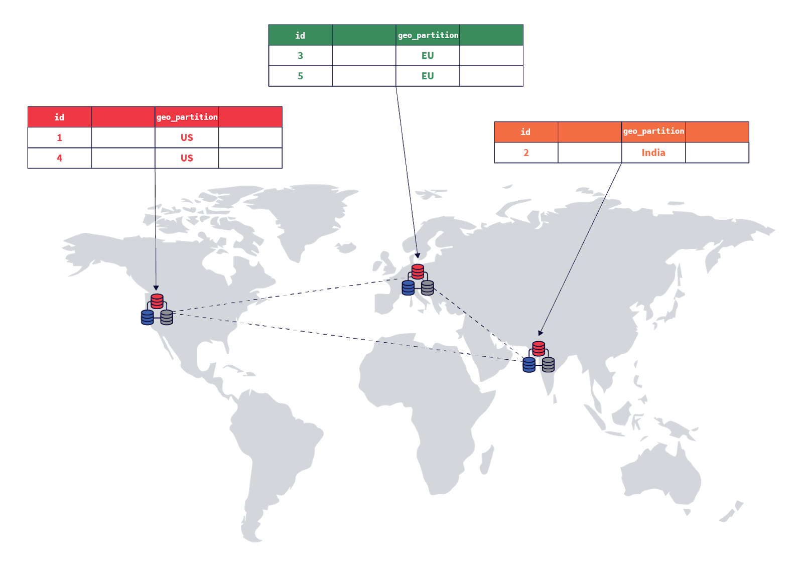
The data is now arranged as follows:

system.transactions_90141438-f42c-4a39-8a12-4072c1216d46.Step 3. Pin user partitions specific to geographic locations
Now, the setup should automatically be able to pin rows to the appropriate regions based on the value set in the geo_partition column. This is shown in the following diagram:

You can test this region pinning by inserting a few rows of data and verifying they are written to the correct partitions.
The sample output includes expanded auto mode output formatting for better readability. You can enable this mode with the following statement:
yugabyte=# \x auto
Expanded display is used automatically.
-
Insert a row into the table with the
geo_partitioncolumn value set toEUbelow.INSERT INTO bank_transactions VALUES (100, 10001, 'EU', 'checking', 120.50, 'debit'); -
Verify that the row is present in the
bank_transactionstable.yugabyte=# select * from bank_transactions;-[ RECORD 1 ]-+--------------------------- user_id | 100 account_id | 10001 geo_partition | EU account_type | checking amount | 120.5 txn_type | debit created_at | 2020-11-07 21:28:11.056236
Additionally, the row must be present only in the bank_transactions_eu partition, which can be easily verified by running the select statement directly against that partition. The other partitions should contain no rows.
yugabyte=# select * from bank_transactions_eu;
-[ RECORD 1 ]-+---------------------------
user_id       | 100
account_id    | 10001
geo_partition | EU
account_type  | checking
amount        | 120.5
txn_type      | debit
created_at    | 2020-11-07 21:28:11.056236
yugabyte=# select count(*) from bank_transactions_india;
 count
-------
     0
yugabyte=# select count(*) from bank_transactions_us;
 count
-------
     0
Insert data into the other partitions.
INSERT INTO bank_transactions
    VALUES (200, 20001, 'India', 'savings', 1000, 'credit');
INSERT INTO bank_transactions
    VALUES (300, 30001, 'US', 'checking', 105.25, 'debit');
These can be verified as follows:
yugabyte=# select * from bank_transactions_india;
-[ RECORD 1 ]-+---------------------------
user_id       | 200
account_id    | 20001
geo_partition | India
account_type  | savings
amount        | 1000
txn_type      | credit
created_at    | 2020-11-07 21:45:26.011636
yugabyte=# select * from bank_transactions_us;
-[ RECORD 1 ]-+---------------------------
user_id       | 300
account_id    | 30001
geo_partition | US
account_type  | checking
amount        | 105.25
txn_type      | debit
created_at    | 2020-11-07 21:45:26.067444
Step 4. Query the local partition
Querying from a particular partition can be accomplished by using a WHERE clause on the partition key. For example, if the client is in the US, querying the local partition can be done by running the following query:
yugabyte=# select * from bank_transactions where geo_partition='US';
-[ RECORD 1 ]-+---------------------------
user_id       | 300
account_id    | 30001
geo_partition | US
account_type  | checking
amount        | 105.25
txn_type      | debit
created_at    | 2020-11-07 21:45:26.067444
However, if you need to query the local partition without specifying the partition column, you can use the function yb_is_local_table. To implement the same query as above using yb_is_local_table, you can do the following:
yugabyte=# select * from bank_transactions where yb_is_local_table(tableoid);
-[ RECORD 1 ]-+---------------------------
user_id       | 300
account_id    | 30001
geo_partition | US
account_type  | checking
amount        | 105.25
txn_type      | debit
created_at    | 2020-11-07 21:45:26.067444
Step 5. Users travelling across geographic locations
To make things interesting, say user 100, whose first bank transaction was performed in the EU region, travels to India and the US, and performs two other bank transactions. This can be simulated by using the following statements:
INSERT INTO bank_transactions
    VALUES (100, 10001, 'India', 'savings', 2000, 'credit');
INSERT INTO bank_transactions
    VALUES (100, 10001, 'US', 'checking', 105, 'debit');
Now, each of the bank transactions would be pinned to the appropriate geographic locations. This can be verified as follows.
yugabyte=# select * from bank_transactions_india where user_id=100;
-[ RECORD 1 ]-+---------------------------
user_id       | 100
account_id    | 10001
geo_partition | India
account_type  | savings
amount        | 2000
txn_type      | credit
created_at    | 2020-11-07 21:56:26.760253
yugabyte=# select * from bank_transactions_us where user_id=100;
-[ RECORD 1 ]-+---------------------------
user_id       | 100
account_id    | 10001
geo_partition | US
account_type  | checking
amount        | 105
txn_type      | debit
created_at    | 2020-11-07 21:56:26.794173
All the bank transactions made by the user can be retrieved using the following SQL statement.
yugabyte=# select * from bank_transactions where user_id=100 order by created_at desc;
-[ RECORD 1 ]-+---------------------------
user_id       | 100
account_id    | 10001
geo_partition | US
account_type  | checking
amount        | 105
txn_type      | debit
created_at    | 2020-11-07 21:56:26.794173
-[ RECORD 2 ]-+---------------------------
user_id       | 100
account_id    | 10001
geo_partition | India
account_type  | savings
amount        | 2000
txn_type      | credit
created_at    | 2020-11-07 21:56:26.760253
-[ RECORD 3 ]-+---------------------------
user_id       | 100
account_id    | 10001
geo_partition | EU
account_type  | checking
amount        | 120.5
txn_type      | debit
created_at    | 2020-11-07 21:28:11.056236
Step 6. Add a new geographic location
Assume that after a while, Yuga Bank gets a lot of customers across the globe, and wants to offer the service to residents of Brazil, which also has data residency laws. Using row-level geo-partitioning, you can do this by adding a new partition and pinning it to the AWS South America (São Paulo) region sa-east-1.
First, create the tablespace:
CREATE TABLESPACE sa_east_1_tablespace WITH (
    replica_placement='{"num_replicas": 3, "placement_blocks":
      [{"cloud":"aws","region":"sa-east-1","zone":"sa-east-1a","min_num_replicas":1},
      {"cloud":"aws","region":"sa-east-1","zone":"sa-east-1b","min_num_replicas":1},
      {"cloud":"aws","region":"sa-east-1","zone":"sa-east-1c","min_num_replicas":1}]}'
    );
Then, create the partition for Brazil:
CREATE TABLE bank_transactions_brazil
    PARTITION OF bank_transactions
      (user_id, account_id, geo_partition, account_type,
       amount, txn_type, created_at,
       PRIMARY KEY (user_id HASH, account_id, geo_partition))
    FOR VALUES IN ('Brazil') TABLESPACE sa_east_1_tablespace;
And with that, the new region is ready to store bank transactions of the residents of Brazil.
INSERT INTO bank_transactions
    VALUES (400, 40001, 'Brazil', 'savings', 1000, 'credit');

select * from bank_transactions_brazil;
-[ RECORD 1 ]-+-------------------------
user_id       | 400
account_id    | 40001
geo_partition | Brazil
account_type  | savings
amount        | 1000
txn_type      | credit
created_at    | 2020-11-07 22:09:04.8537
Step 7. Fault tolerance during a region outage
So far you've set up replication with 3 copies of the data, which helps tolerate the loss of a single node or zone. However, a regional outage will cause unavailability, because all the nodes are in one region. Placing each replica in a different region helps solve this issue.
Recreate the us_west_2_tablespace from earlier, and place one copy each in us-west2, us-west1, and us-east1. Then use leader_preference to continue placing all leaders in us-west-2, so that they remain close to the client and provide the best performance. (You can find more information in Leader preference)
CREATE TABLESPACE us_west_2_tablespace WITH (
  replica_placement='{"num_replicas": 3, "placement_blocks":
  [{"cloud":"aws","region":"us-west-2","zone":"us-west-2a","min_num_replicas":1,"leader_preference":1},
  {"cloud":"aws","region":"us-west-1","zone":"us-west-1a","min_num_replicas":1,"leader_preference":2},
  {"cloud":"aws","region":"us-east-1","zone":"us-east-1a","min_num_replicas":1}]}'
);
Write latency
Having the client and leader in the same zone reduces network roundtrip between them. The read latency will be similar to having all replicas in the same zone, and the write latency will be slightly higher, as the quorum commit needs to wait for data to get replicated to a different region.